Compound probability distribution

In probability theory, a compound probability distribution is the probability distribution that results from assuming that a random variable is distributed according to some parametrized distribution $F$ with an unknown parameter θ that is distributed according to some other distribution G, and then determining the distribution that results from marginalizing over G (i.e. integrating the unknown parameter out). The resulting distribution H is said to be the distribution that results from compounding F with G. In Bayesian inference, the distribution G is often a conjugate prior of F.

Examples

Compounding a Gaussian distribution with mean distributed according to another Gaussian distribution yields a Gaussian distribution.
Compounding a Gaussian distribution with precision (reciprocal of variance) distributed according to a gamma distribution yields a three-parameter Student's t distribution.
Compounding a binomial distribution with probability of success distributed according to a beta distribution yields a beta-binomial distribution.
Compounding a multinomial distribution with probability vector distributed according to a Dirichlet distribution yields a multivariate Pólya distribution, also known as a Dirichlet compound multinomial distribution.
Compounding a gamma distribution with inverse scale parameter distributed according to another gamma distribution yields a three-parameter beta prime distribution.

Theory

Note that the support of the resulting compound distribution $H$ is the same as the support of the original distribution $F$ . For example, a beta-binomial distribution is discrete just as the binomial distribution is (however, its shape is similar to that of a beta distribution). The variance of the compound distribution $H$ is typically greater than the variance of the original distribution $F$ . The parameters of $H$ include the parameters of $G$ and any parameters of $F$ that are not marginalized out. For example, the beta-binomial distribution includes three parameters, a parameter $n$ (number of samples) from the binomial distribution and shape parameters $\alpha$ and $\beta$ from the beta distribution.

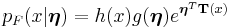
Note also that, in general, the probability density function of the result of compounding an exponential family distribution with its conjugate prior distribution can be determined analytically. Assume that $F(x|\boldsymbol{\theta})$ is a member of the exponential family with parameter $\boldsymbol{\theta}$ that is parametrized according to the natural parameter $\boldsymbol{\eta} = \boldsymbol{\eta}(\boldsymbol{\theta})$ , and is distributed as

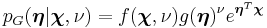
$p_F(x|\boldsymbol{\eta}) = h(x)g(\boldsymbol{\eta})e^{\boldsymbol{\eta}^T\mathbf{T}(x)}$

while $G(\boldsymbol{\eta}|\boldsymbol{\chi},\nu)$ is the appropriate conjugate prior, distributed as

$p_G(\boldsymbol{\eta}|\boldsymbol{\chi},\nu) = f(\boldsymbol{\chi},\nu)g(\boldsymbol{\eta})^\nu e^{\boldsymbol{\eta}^T\boldsymbol{\chi}}$

Then the result $H$ of compounding $F$ with $G$ is

$\begin{align} p_H(x|\boldsymbol{\chi},\nu) &= {\displaystyle \int\limits_\boldsymbol{\eta} p_F(x|\boldsymbol{\eta}) p_G(\boldsymbol{\eta}|\boldsymbol{\chi},\nu) \,\operatorname{d}\boldsymbol{\eta}} \\ &= {\displaystyle \int\limits_\boldsymbol{\eta} h(x)g(\boldsymbol{\eta})e^{\boldsymbol{\eta}^T\mathbf{T}(x)} f(\boldsymbol{\chi},\nu)g(\boldsymbol{\eta})^\nu e^{\boldsymbol{\eta}^T\boldsymbol{\chi}} \,\operatorname{d}\boldsymbol{\eta}} \\ &= {\displaystyle h(x) f(\boldsymbol{\chi},\nu) \int\limits_\boldsymbol{\eta} g(\boldsymbol{\eta})^{\nu%2B1} e^{\boldsymbol{\eta}^T(\mathbf{T}(x) %2B \boldsymbol{\chi})} \,\operatorname{d}\boldsymbol{\eta}} \\ &= h(x) \dfrac{f(\boldsymbol{\chi},\nu)}{f(\mathbf{T}(x) %2B \boldsymbol{\chi}, \nu%2B1)} \end{align}$

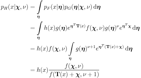
The last line follows from the previous one by recognizing that the function inside the integral is the density function of a random variable distributed as 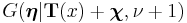$G(\boldsymbol{\eta}|\mathbf{T}(x) %2B \boldsymbol{\chi}, \nu%2B1)$ , excluding the normalizing function $f(\dots)\,$ . Hence the result of the integration will be the reciprocal of the normalizing function.

The above result is independent of choice of parametrization of $\boldsymbol{\theta}$ , as none of $\boldsymbol{\theta}$ , $\boldsymbol{\eta}$ and $g(\dots)\,$ appears. (Note that $g(\dots)\,$ is a function of the parameter and hence will assume different forms depending on choice of parametrization.) For standard choices of $F$ and $G$ , it is often easier to work directly with the usual parameters rather than rewrite in terms of the natural parameters.

Note also that the reason the integral is tractable is that it involves computing the normalization constant of a density defined by the product of a prior distribution and a likelihood. When the two are conjugate, the product is a posterior distribution, and by assumption, the normalization constant of this distribution is known. As shown above, the density function of the compound distribution follows a particular form, consisting of the product of the function $h(x)$ that forms part of the density function for $F$ , with the quotient of two forms of the normalization "constant" for $G$ , one derived from a prior distribution and the other from a posterior distribution. The beta-binomial distribution is a good example of how this process works.

Despite the analytical tractability of such distributions, they are in themselves usually not members of the exponential family. For example, the three-parameter Student's t distribution, beta-binomial distribution and Dirichlet compound multinomial distribution are not members of the exponential family. This can be seen above due to the presence of functional dependence on $\mathbf{T}(x) %2B \boldsymbol{\chi}$ . In an exponential-family distribution, it must be possible to separate the entire density function into multiplicative factors of three types: (1) factors containing only variables, (2) factors containing only parameters, and (3) factors whose logarithm factorizes between variables and parameters. The presence of $\mathbf{T}(x) %2B \boldsymbol{\chi}$ makes this impossible unless the "normalizing" function $f(\dots)\,$ either ignores the corresponding argument entirely or uses it only in the exponent of an expression.

It is also possible to consider the result of compounding a joint distribution over a fixed number of independent identically distributed samples with a prior distribution over a shared parameter. When the distribution of the samples is from the exponential family and the prior distribution is conjugate, the resulting compound distribution will be tractable and follow a similar form to the expression above. It is easy to show, in fact, that the joint compound distribution of a set 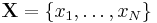$\mathbf{X} = \{x_1, \dots, x_N\}$ for $N$ observations is

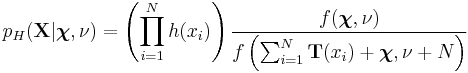
$p_H(\mathbf{X}|\boldsymbol{\chi},\nu) = \left( \prod_{i=1}^N h(x_i) \right) \dfrac{f(\boldsymbol{\chi},\nu)}{f\left(\sum_{i=1}^N \mathbf{T}(x_i) %2B \boldsymbol{\chi}, \nu%2BN \right)}$

This result and the above result for a single compound distribution extend trivially to the case of a distribution over a vector-valued observation, such as a multivariate Gaussian distribution.

A related but slightly different concept of "compound" occurs with the compound Poisson distribution. In one formulation of this, the compounding takes places over a distribution resulting from N underlying distributions, in which N is itself treated as a random variable. The compound Poisson distribution results from considering a set of independent identically-distributed random variables distributed according to J and asking what the distribution of their sum is, if the number of variables is itself an unknown random variable $N$ distributed according to a Poisson distribution and independent of the variables being summed. In this case the random variable N is marginalized out much like θ above is marginalized out.

Compound probability distribution

Examples

Theory

References